Steven S. Skiena
Dept. of Computer Science
SUNY Stony Brook
Many problems in both finance and computer science reduce to trying to predict the future...
Examples from computer science include cache and virtual memory management.
Examples from finance typically revolve around predicting future returns for an asset, or designing a portfolio to maximize future returns.
Such problems become trivial if we know the future (i.e. the stream of future memory requests or tomorrow's newspaper), but typically we only have access to the past.
An off-line problem provides access to all the relevant information to compute a result.
An online problem continually produces new input and requires answers in response.
How can we theoretically evaluate how well an algorithm forecasts the future?
Statistical forecasts provide a predict the future that makes some sense in practice. However, they offer no future guarantees, particularly if the data distribution changes.
Competitive analysis offers a worst-case measure of the quality of the behavior of an algorithm which predicts the future.
We seek to compare the performance of algorithm ![]() with only knowledge of
the past with an algorithm which has complete knowledge of past and future
makes optimal use of it.
with only knowledge of
the past with an algorithm which has complete knowledge of past and future
makes optimal use of it.
We say an online algorithm ![]() is
is ![]() -competitive if there is a
constant
-competitive if there is a
constant ![]() such that for all finite input sequences
such that for all finite input sequences ![]() ,
,
Note that the additive constant ![]() is a fixed cost that
becomes unimportant as the size of the problem increases.
is a fixed cost that
becomes unimportant as the size of the problem increases.
We do not particularly care about the run-time efficiency of ![]() (except maybe that it is polynomial), but we do care about its
competitive ratio
(except maybe that it is polynomial), but we do care about its
competitive ratio ![]() .
.
Consider the problem of deciding when to purchase skis.
Whenever you go skiing, you can either rent skis for the day at cost ![]() ,
or buy them for
,
or buy them for ![]() .
.
If you buy them the first day, the worst case is you never ski again,
and you spent ![]() times the optimal decision of simply renting.
times the optimal decision of simply renting.
Suppose you never buy them. After ![]() days, you have spent
days, you have spent ![]() times
the optimal decision of buying from the first day.
times
the optimal decision of buying from the first day.
But suppose you buy them after renting ![]() times.
times.
You did the right thing if you go ![]() times.
If you go exactly
times.
If you go exactly ![]() times, you spent twice as much as the optimal decision,
but never changes after that.
times, you spent twice as much as the optimal decision,
but never changes after that.
Thus this ``balancing'' algorithm is ![]() -competitive.
-competitive.
We can view any online algorithm as a game between an online player (the skier) and a malicious adversary (his/her anterior cruciate ligament).
Suppose that we want to sell a indivisible asset (say a house)
sometime over the next ![]() days.
days.
Say the price fluctuates on a daily basis in the real interval
![]() , where
, where ![]() is the lowest possible price and
is the lowest possible price and ![]() is the highest
possible price.
is the highest
possible price.
What strategy can we use to sell the asset and get the highest possible price?
If we knew the future history, the optimal strategy would be to that
the maximum price occurring over the ![]() days.
days.
We seek a strategy which optimizes competitive ratio, i.e. which minimizes the maximum ratio of the price we get over the maximum price.
We do not seek a price which is good related to the ``average'', but good in the worst case.
What can we do?
Note that if the price was high at one point but we didn't sell,
our adversary could immediately and permanently lower the price to ![]() .
.
Note that once we sell, our adversary can immediately raise the price
to ![]() .
.
At the end of the time period, we can always get a price of at least ![]() .
.
Together, this suggests that we should buy the instant the price reaches
some ![]() which is high enough that we do OK in each instance.
which is high enough that we do OK in each instance.
The worst we do in the first case is ![]() .
The worst we do in the second case is
.
The worst we do in the second case is ![]() .
Balancing them yields:
.
Balancing them yields:
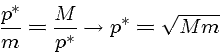
The reservation price policy (RPP) accepts the first price greater
than or equal to
![]() .
.
Let ![]() define the global fluctuation ratio.
define the global fluctuation ratio.
The competitive ratio ![]() we get is
we get is
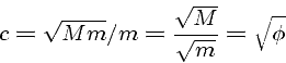
This is the optimal deterministic strategy.
Randomized algorithms use random numbers to help them make decisions.
Randomization is particularly useful to make things difficult for an adversary - we assume the adversary has access to your program to design a future that is bad for you, but does not have access to read or effect the random numbers.
In an analysis of a randomized algorithms, we determine the expected value over all random number sequences for the worst possible input.
Thus our analysis is completely independent of the input distribution - randomized expectation has nothing to do with statistical expectation.
Randomization can be used to design simple algorithms which make it unlikely to encounter the worst possible case.
Suppose I ride over a tack and get a flat tire.
What is the best way I can find the location of the tack, assuming I can
only explore ![]() th of the wheel at a time?
th of the wheel at a time?
Suppose I use the deterministic
strategy of repeatedly turning the wheel left
![]() radians until I find the tack.
radians until I find the tack.
But my adversary can put the tack just to the right of the initial position.
Then strategy yields a cost of ![]() versus the optimal off-line cost of 1,
for a competitive ratio of
versus the optimal off-line cost of 1,
for a competitive ratio of ![]() .
.
Suppose instead I spin the wheel around randomly and then start walking
to the left.
Regardless of where the adversary puts the tack, my expected search cost
(and competitive ratio) is ![]() .
.
Suppose that
![]() for some integer
for some integer ![]() , i.e.
, i.e. ![]() .
.
Let ![]() be the deterministic reservation price policy where
we buy soon at the price hits
be the deterministic reservation price policy where
we buy soon at the price hits ![]() .
.
The strategy ![]() picks an integer
picks an integer ![]() uniformly at random
from
uniformly at random
from ![]() , and then performs buys soon iff the price hits
, and then performs buys soon iff the price hits ![]() .
.
There must be some ![]() such that the optimum off-line return
such that the optimum off-line return ![]() lies between
lies between
![]() .
.
What can the adversary do?
Knowing we are restricted to picking values of the form ![]() ,
they will pick a value of the form
,
they will pick a value of the form
![]() to frustrate us for some
to frustrate us for some ![]() .
.
Suppose the adversary picks ![]() .
.
Our target ![]() was too big with probability
was too big with probability ![]() - if so we were
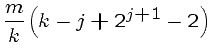
forced to settle for a price of
- if so we were
forced to settle for a price of ![]() .
.
Our target ![]() was less than
was less than ![]() otherwise, meaning were able
to realize our price.
otherwise, meaning were able
to realize our price.
Our expected price is:
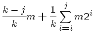 |
(1) | ||
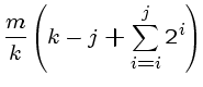 |
(2) | ||
 |
(3) |
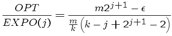
The competitive ratio is
 |
(4) | ||
 |
(5) |
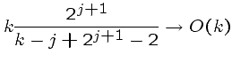
The competitive ratio is maximized when ![]() is largest, for a
competitive ratio of
is largest, for a
competitive ratio of ![]() .
.
A generalization of the price searching problem is to sell my entire assets over the trading period, but to remove the constraint that I must sell it all at once.
Suppose I am trying to liquidate my position in a stock. I may be able to better optimize my expected performance by using this freedom.
This is particularly true in real markets, as my sales serve to depress prices by increasing supply.
For this problem, it turns out that there is no difference between what competitive ratio is achievable with and without randomization.
What is a reasonable strategy?
Suppose we know that a competitive ratio of ![]() can be obtained.
can be obtained.
If the current price is high and I don't sell, my adversary can drop it
to ![]() and keep it there the rest of the period.
and keep it there the rest of the period.
But if I do buy, the adversary can jack the price to ![]() at least momentarily,
and I will be in trouble if I have already sold everything.
at least momentarily,
and I will be in trouble if I have already sold everything.
The threat-based strategy buys only when the price hits a new
maximum.
It buys just enough to ensure that we achieve a competitive ratio of ![]() if the price drops to
if the price drops to ![]() for the rest of the game.
for the rest of the game.
Analysis is needed to determine the optimal ![]() value and also
how much to buy in response to price changes.
value and also
how much to buy in response to price changes.
Clearly, we can achieve
![]() , since we can use the randomized
strategy and sell all at once.
, since we can use the randomized
strategy and sell all at once.
Note that we can simulate the randomized strategy deterministically by
putting ![]() th of our money on each value of
th of our money on each value of ![]() .
.
The optimal
threat-based strategy for one-way trading achieves a competitive ratio
of
![]() times better the search bound of
times better the search bound of ![]() .
.
How useful are our competitive algorithms for price searching and one-way trading?
Our assumptions of upper and lower bounds on possible price movements seem suspicious, although one can probably make save over/under-estimates of possible movements over short periods of time using historical data.
Still, wider upper/lower price bounds imply worse competitive ratios.
Guaranteeing you do, say half, as well as optimal doesn't look so good when the difference between the best investor and an index fund is often only a few percentage points.
That said, the randomized and threat-based heuristics seem to suggest reasonable approaches for one-way trading.
Suppose we can invest in a market with ![]() types of assets,
including cash.
types of assets,
including cash.
How should partition our money among the assets, and how should we adjust our portfolio to changes in asset prices?
The buy and hold strategy (BAH) strategy does not attempt to modify the portfolio for long periods of time.
Buy and hold results in very low transaction costs, and is historically better for individual investors to do than market-timing strategies which switch among investments seeking the best return.
Of course, market timing can yield much better returns if
you do it right.
Consider a stock that alternates returns of ![]() and
and ![]() .
Buy and hold returns at most
.
Buy and hold returns at most ![]() over any period of length
over any period of length ![]() , while
the optimal market timing would yield a return of
, while
the optimal market timing would yield a return of ![]() .
.
A constant rebalancing algorithm always puts ![]() of our current
wealth in each of the
of our current
wealth in each of the ![]() securities.
securities.
Such a diversified strategy enables us to pickup exponential growth over the previous return sequence if it starts positively.
Implementing a constant rebalancing strategy requires daily trades, but provides a way to capitalize on boom periods.
Two-way trading is a special case of online portfolio selection where you have only cash and one other security you can hold.
It differs from one-way trading in that we can shift back and forth between the two assets.
The optimal offline strategy is clear: put all your assets into the security on any day it offers positive returns. Otherwise, put everything into cash.
A trading strategy is said to be money making if it returns positive profit on every market sequence for which the optimal offline algorithm makes a profit.
The general adversary can ensure that no money making strategy exists.
If you are not initially invested in the non-cash asset, the next period will be the only one offering positive returns. If you are initially invested in the non-cash asset, offer such a negative return as to essentially wipe it out, then have a small enough positive return that you cannot recoup what you lost.
Money making strategies are only possible against weaker adversaries.
An ![]() trading sequence is a
trading sequence is a ![]() day sequence of returns for
which the optimal offline strategy generates a return of at least
day sequence of returns for
which the optimal offline strategy generates a return of at least ![]() .
.
An ![]() adversary is constrained to produce
adversary is constrained to produce ![]() trading
sequences.
trading
sequences.
We assume that you are given ![]() and
and ![]() in advance to help you
plan your trading strategy.
in advance to help you
plan your trading strategy.
Can you devise a provably money making strategy against
an ![]() adversary?
adversary?
How about when ![]() ?
?
How about when ![]() ?
?
For ![]() , we have only one trading period.
Since this must produce a profit
, we have only one trading period.
Since this must produce a profit ![]() , we should be fully
invested in the non-cash asset.
, we should be fully
invested in the non-cash asset.
For ![]() , we must look ahead to the case of
, we must look ahead to the case of ![]() .
If we initially bet only on cash, the adversary will make that the only
period of positive return.
.
If we initially bet only on cash, the adversary will make that the only
period of positive return.
If we are initially out of cash, the adversary can wipe us out now and
show a ![]() in the next period.
in the next period.
We must bet something but not everything on the non-cash asset in
the first round.
If it shows positive return, we can quite the game with our holdings.
If it shows negative return, we still have money and know there must
be a positive return of at least ![]() in the remaining time.
in the remaining time.
Through such reasoning, for large ![]() we can work backwards from
we can work backwards from ![]() to figure out the best first move to make.
to figure out the best first move to make.
If ![]() , invest in the non-cash asset for return
, invest in the non-cash asset for return ![]() .
.
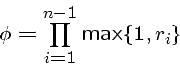
Otherwise, invest the fraction ![]() of your wealth in the non-cash asset, where
of your wealth in the non-cash asset, where
![]() returns the
returns the ![]() which maximizes the value, as opposed to
which maximizes the value, as opposed to
![]() which returns the value.
which returns the value.
Once you pick a ![]() , your adversary will pick a return
, your adversary will pick a return ![]() such as to minimize
your wealth.
such as to minimize
your wealth.
Your wealth after this event is your initial wealth times the returns
on the cash and non-cash portions, i.e. ![]() .
.
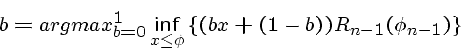
After the return ![]() is revealed to you, you can figure out the
guaranteed return for the remaining period:
is revealed to you, you can figure out the
guaranteed return for the remaining period:
The best value of ![]() can be determined by dynamic programming.
can be determined by dynamic programming.
Although this strategy is provably money-making, its
can be yield poor returns for large ![]() ,
,
For large ![]() , it can initially only afford to put a small amount of money into
non-cash assets.
, it can initially only afford to put a small amount of money into
non-cash assets.
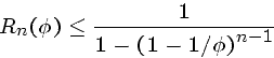
Since the optimal offline return is ![]() , we get a not-inspiring
competitive ratio
of
, we get a not-inspiring
competitive ratio
of
![]() .
.