CSE 691 - Lecture 7 - Linear Time Series Analysis

Steven S. Skiena

Dept. of Computer Science

SUNY Stony Brook

Covariance and Correlation

The covariance of random variables $X$ and $Y$, is defined

$$\mbox{Cov}(X,Y) = E[ (X - \mu_x)(Y - \mu_y) ]$$

If $X$ and $Y$ are ``in sync'' the covariance will be high; if they are independent, positive and negative terms should cancel out to give a score around zero.

The lag-$l$ auto-covariance $\mbox{Cov}(r_t,r_{t-l}) = \gamma_l$ has two interesting properties, (1) $\gamma_0 = Var(r_t)$ and (2) $gamma_l = \gamma_{-l}$.

The correlation coefficient of random variables $X$ and $Y$, is defined

$$\rho_{x,y} = \frac{\mbox{Cov}(X,Y)}{\sqrt{ Var(X) Var(Y) }}$$

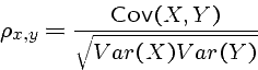
It measures the strength of linear dependence between $X$ and $Y$, and lies between -1 and 1.

Correlation and Causation

Note that correlation does not imply causation - the conference of the Super Bowl winner has had amazing success predicting the fate of the stock market that year.

If you investigate the correlation of many pairs of variables (such as in data mining), some are destined to have high correlation by chance.

The meaningfulness of the correlation can be evaluated by considering (1) the number of pairs tested, (2) the number of points in each time series, (3) the sniff test of whether there should be a connection, (4) statistical tests.

Stationarity

The mathematical tools we apply to the analysis of time series data rest on certain assumptions about the nature of the time series.

A time series $\{r_t\}$ is said to be weakly stationary if (1) the mean of $r_t$, $E(r_t)$, is a constant and (2) the covariance $\mbox{Cov}(r_t,r_{t-l}) = \gamma_l$, which depends only upon $l$.

In a weakly stationary series, the data values fluctuate with constant variation around a constant level.

The financial literature typically assumes that asset returns are weakly stationary, as can be tested empirically.

Autocorrelation

The lag-$l$ autocorrelation $\rho_l$ is the correlation coefficient of $r_t$ and $r_{t-l}$.

A linear time-series is characterized by its sample autocorrelation function ${a_l} = \rho_l$.

The naive algorithm for computing the autocorrelation function takes $O(n^2)$ time for a series of $n$ terms, however fast convolution algorithms can compute it in $O(n \log n)$ time.

What would we expect the autocorrelation function of stock returns to look like?

If stock returns are truly random, we expect all lags to show a correlation of around zero.

What about stock market volatility?

Presumably today's volatility is a good predictor for tomorrow, so we expect high autocorrelations for short lags.

What about daily gross sales for Walmart?

Presumably today's sales are a good predictor for yesterday's, so we expect high autocorrelations for short lags.

However, there are presumably also day-of-week effects (Sunday is a bigger sales day than Monday) and day-of-year effects (Christmas season is bigger than mid-summer). These will show up as lags of 7 and about 365, respectively.

Autocorrelation Analysis of GDP

**** Demonstration of Analysis of U.S. Quarterly Real GDP: 1967-2002.
**** "<====" indicates my explanation of the command.
**** Output will be explained in class.
 --
input x1,x. file 'q-rgdpf6702.dat'   <=== Load data into SCA.

 X1      , A  144  BY   1 VARIABLE, IS STORED IN THE WORKSPACE
 X       , A  144  BY   1 VARIABLE, IS STORED IN THE WORKSPACE
 --
y=ln(x)    <=== Take natural log transformation
 --
diff old y. new dy. comp.   <=== Take first difference of the log series.

                             1
 DIFFERENCE ORDERS ARE  (1-B  ) 
 SERIES    Y     IS DIFFERENCED, THE RESULT IS STORED IN VARIABLE    DY   
 SERIES    DY    HAS  143  ENTRIES
 --
iden dy.    <=== Compute ACF and PACF of the differenced series.

 NAME OF THE SERIES . . . . . . . . . .           DY
 TIME PERIOD ANALYZED . . . . . . . . .  1  TO   143
 MEAN OF THE (DIFFERENCED) SERIES . . .       0.0071
 STANDARD DEVIATION OF THE SERIES . . .       0.0079
 T-VALUE OF MEAN (AGAINST ZERO) . . . .      10.7080

 AUTOCORRELATIONS 

   1- 12     .29  .22  .07  .05 -.06 -.04 -.10 -.23 -.03 -.02 -.01 -.18
   ST.E.     .08  .09  .09  .09  .09  .10  .10  .10  .10  .10  .10  .10
    Q       12.4 19.8 20.4 20.9 21.4 21.7 23.2 31.1 31.3 31.3 31.4 36.5

  13- 24    -.09 -.18 -.13 -.00 -.05  .02  .05  .09  .07  .05 -.01 -.02
   ST.E.     .10  .10  .10  .11  .11  .11  .11  .11  .11  .11  .11  .11
    Q       37.9 43.1 45.7 45.7 46.1 46.2 46.5 47.9 48.7 49.2 49.2 49.3

           -1.0 -0.8 -0.6 -0.4 -0.2  0.0  0.2  0.4  0.6  0.8  1.0
             +----+----+----+----+----+----+----+----+----+----+
                                      I
   1   0.29                       +   IXXX+XXX                  
   2   0.22                       +   IXXX+XX                   
   3   0.07                      +    IXX  +                    
   4   0.05                      +    IX   +                    
   5  -0.06                      +   XI    +                    
   6  -0.04                      +   XI    +                    
   7  -0.10                      + XXXI    +                    
   8  -0.23                     X+XXXXI    +                    
   9  -0.03                      +   XI    +                    
  10  -0.02                      +   XI    +                    
  11  -0.01                      +    I    +                    
  12  -0.18                      +XXXXI    +                    
  13  -0.09                      +  XXI    +                    
  14  -0.18                      XXXXXI    +                    
  15  -0.13                      + XXXI    +                    
  16   0.00                      +    I    +                    
  17  -0.05                      +   XI    +                    
  18   0.02                      +    IX   +                    
  19   0.05                      +    IX   +                    
  20   0.09                      +    IXX  +                    
  21   0.07                      +    IXX  +                    
  22   0.05                      +    IX   +                    
  23  -0.01                      +    I    +                    
  24  -0.02                      +   XI    +

Thus autocorrelation analysis enables us to identify periodic cycles in the time series.

Autoregressive Models

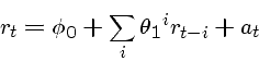
A simple autoregressive model to capture a significant lag-1 autocorrelation is

$$r_t = \phi_0 + \phi_1 r_{t-1} + a_t$$

where $\{a_t\}$ is assumed to be a white noise series with mean zero and ${\sigma_a}^2$.

The autocorrelation function of white noise should be near zero.

The order of the model is the number of terms of history; this is an $AR(1)$ model, which can readily be generalized into $AR(p)$ models for arbitrary $p$.

Building Autoregressive Models

For a given return series and desired history, the $\phi_i$ parameters can be found using the least squares method.

Build an $(n-p) \times (p+1)$ matrix where the $l$th column is the lag-$(l-1)$ return series.

If $p \approx n$, we have a complete linear system, and Gaussian elimination will set all of the parameters.

When $p \leq n$, we can find the $\phi$ coefficients which minimize least-square errors.

The white noise residual terms can be calculated

$$a_t = r_t - ( \phi_0 + \phi_1 r_{t-1} )$$

A model is likely good if the magnitude and variance of the residual terms are small.

A model has likely captured enough history if the autocorrelation function of the residuals is small.

Forecasting with Autoregressive Models

The value of the model at the next time step can be easily predicted by plugging in terms.

$$r_t = \phi_0 + \phi_1 r_{t-1}$$

The observed variance of the residual terms provides error bounds on the reliability of our forecast.

By plugging the predicted next value into the model and repeating, we can forecast indefinitely into the future but the error bounds on our predictions will deteriorate.

Moving Average Models

A special class of autoregressive models assumes complete history, but constrains the coefficients to make the number of parameters tractable.

The form of an exponentially weighted moving average model is

$$r_t = \phi_0 + \sum_i {\theta_1}^i r_{t-i} + a_t$$

Note that the weight of each term decreases exponentially with history.

Subtracting the series for $r_t$ and $\theta_1 r_{t-1}$ yields

$$r_t = \phi_0(1-\theta_1) + a_t - \theta_1 a_{t-1}$$

Thus the next prediction of $r_t$ from such an order-1 moving average model can be computed from the previous prediction and the next result.

In general, an $MA(q)$ model has form

$$r_t = c_0 + a_t - \sum_i^{i=q} \theta_q a_{t-q}$$

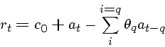
The order of such a model can be determined by analysis of the autocorrelation function.

The parameters of this model cannot be set using least squares, because the error terms $a_t$ are affected by the parameters themselves.

Trial and error (for $MA(1)$ models) or more sophisticated numerical methods are needed.

Exponential moving average models are often used for volatility prediction,

$$V_n = \lambda V_{n-1} + (1 - \lambda) V'_{n-1}$$

where $V$ is the predicting volatility and $V'$ the observed volatility.

Volatility is fairly stable, as shown by the fact that the last 30 to 90 days still has predictive power. Thus the exponential decay must be small. The RiskMetrics model uses $\lambda \approx 0.944$ for volatility estimation.

Relating Time Series

In many applications, the relationship between two time series is important.

Consider the relationship between the 1-year Treasury interest rate $r_{1t}$ and the 3-year rate $r_{3t}$, sampled each week.

We expect them both to move pretty much in tandem in response to world events, and that typically $r_{3t} > r_{1t}$. But what is the relationship?

A simple linear model yields

$$r_{3t} = \alpha + \beta r_{1t} + e_t$$

where $e_t$ is the error term.

When fitted to data, this yielded

$$r_{3t} = 0.911 + .924 r_{1t} + e_t$$

with $\sigma_e = 0.538$ and $R^2=95.8$%.

However, if we plot the error terms, we see these residuals are highly autocorrelated - there are periods in time where the yield curve is inverted.

The high serial correlation and $R_2$ are misleading; there is not a long-term equilibrium between the rates.

Since our residuals are not independent, we must look for a model which removes such autocorrelations.

Removing Autocorrolations

Consider the delta functions $c_{1t} = r_{1t} - r_{1,t-1}$ and $c_{3t} = r_{3t} - r_{3,t-1}$

These deltas remain highly correlated, since

$$c_{3t} = 0.0002 + 0.7811 c_{1t} + e_t$$

with $\sigma_e = 0.0682$ and $R^2=84.8$%.

However, the remaining error terms are not significantly autocorrelated.

We can use a moving average ($MA(1)$) model to remove such autocorrelations,

$$c_{3t} = \alpha + \beta r_{3t} + a_t - \theta a_{t-1}$$

The parameters can be fit using maximum likelihood methods.

Once such parameters are fit, the delta functions can be back substituted to give us $r_{3t}$ as a function of $r_{3,t-1}$, $r_{1t}$, $r_{1,t-1}$, and $a_{t-1}$.

GARCH Models

We have previously associated the risk of an investment with the volatility of its returns.

The implied volatility of a return series is defined by the variance of the returns.

However, this calculation is based on the assumption that returns are log-normally distributed.

GARCH (generalized autoregressive conditional heteroscedastic) models are often used to model volatility.

Heteroscedastic means a set of statistical distributions having different variances.

Let $a_t = r_t - \mu_t$ The GARCH(1,1) model is defined by $a_t = \sigma_t \epsilon_t$ where

$${\sigma_t}^2 = \alpha_0 + \alpha_1 a_{t-1}^2 + \beta_1 {\sigma_{t-1}}^2$$

where $0 \leq \alpha_1$, $\beta_1 \leq 1$ and $(\alpha_1+\beta_1) < 1$

These conditions imply that the model is mean reverting, which implies that it returns to an average value after reaching extremes.