CSE 691 - Lecture 6 - Financial Time Series Data

Steven S. Skiena

Dept. of Computer Science

SUNY Stony Brook

Time Series Analysis

A time series are the values of a function sampled at different points in time.

Time series data arises throughout the natural and physical sciences, as growth curves, statistical measurements of activity, ...

With respect to financial data, the price of any asset as a function of time naturally gives a time series.

Many relevant statistics (such as the unemployment rate or index of leading economic indicators) can also be thought of as time series data.

A wide variety of mathematical and statistical tools have been developed for working with time series data.

Adherents to technical analysis argue that insight into future price movements follow from the analysis of a given asset's price time series.

Regardless, the analysis of financial time series is important in developing/evaluating any investment strategy, risk modeling, and arbitrage.

Asset Returns

The price of an asset as a function of time is perhaps the most natural financial time series, but it is not the best way to manipulate the data mathematically.

The price of any reasonable asset will increase exponentially with time, but most of our mathematical tools (e.g. correlation, regression) work most naturally with linear functions.

The mean value of an exponentially-increasing time series has no obvious meaning.

The derivative of an exponential function is exponential, so day-to-day changes in price have the same unfortunate properties.

Much better is to represent the data as a simple net return:

$$R_t = \frac{P_t}{P_{t-1}} - 1 = \frac{P_t - P_{t-1}}{P_{t-1}}$$

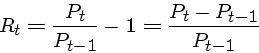
Negative returns means the asset declined in value, positive returns means it increased, zero returns means it is unchanged.

The return is a complete and scale-free summary of investment performance.

Multiperiod Returns

A nice property of returns is that multiplying them gives the return over a longer period:

$$1 + R_t[k] = \frac{P_t}{P_{t-k}} = \prod_{j=0}^{k-1} \frac{P_{t-j}}{P_{t-j-1}} = \prod_{j=0}^{k-1} (1 + R_{t-j})$$

Normally, returns are discussed in annualized terms, so over $k$ years the annualized return is computed by its geometric mean:

$$\{ R_t[k]\} = \left( \prod_{j=0}^{k-1} (1 + R_{t-j}) \right)^{1/k} - 1$$

Why the geometric mean instead of the arithmetic mean? Because $k$ years at the annualized rate of return gives exactly the same payoff as the given return time series.

This can best be computed with logarithms or approximated by its Taylor expansion, an arithmetic mean:

$$\{ R_t[k]\} = \exp \left( \frac{1}{k} \sum_{j=0}^{k-1} \ln(1+... ...-j}) \right) - 1 \approx \frac{1}{k} \sum_{j=0}^{k-1} R_{t-j}$$

Logarithmic and Other Returns

The mathematical complexities of multiplying returns can be eliminated by dealing with continuously compounded returns or log returns:

$$r_t = \ln(1+R_t) = \ln( \frac{P_t}{P_{t-1}} ) = \ln P_t - \ln P_{t-1}$$

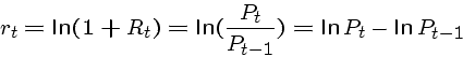
The multiperiod log return is simply the sum of the log returns.

Returns of assets paying dividends must include the value of the dividend payments at the time they are issued. Note that ignoring dividend payments with respect to returns only messes up data points on dividend days, instead of invalidating the entire time series.

The excess return of an asset at time $t$ is the difference between its return and that of a reference asset, typically the risk-free rate.

The excess return is the payoff of a portfolio going long in the asset and short on the reference.

Moments of Distributions

The $l$th moment of a continuous random variable $X$ is defined

$$m'_l = E(X^l) = \int_{-\infty}^{\infty} x^l f(x) dx$$

where $E(X)$ is the expected value and $f(x)$ is the probability density function of $X$.

The first moment is the mean or expectation of $X$, $\mu_x$.

The $l$th central moment of a continuous random variable $X$ is defined

$$m'_l = E(X^l) = \int_{-\infty}^{\infty} (x - \mu_x)^l f(x) dx$$

The second central moment is the variance $(\sigma_x)^2$ where $\sigma_x$ is the standard deviation.

The variance measures how much the random variable jumps around from the mean.

The third central moment is the skewness of the random variable, a measure of the extent of symmetry.

The fourth central moment is the kurtosis, a measure of how much mass in the tails of the distribution.

Properties of Asset Returns

If we consider the returns of a volatile asset, such the daily return on a stock, we would expect:

• The expected value will be small, probably near zero. Think about 10% return divided by 365 days.

• There should be a gross symmetry between negative returns and positive returns.

• Smaller absolute returns will occur more frequently than larger absolute returns.

All of these suggest some time of bell-shaped curve, but which one...

The Normal Distribution

The classic bell-shaped curve is that of the normal distribution, whose probability density function is:

$$f(x)=\frac{e^{((-(x-\mu)^2)/(2 \sigma^2))}}{(\sigma \sqrt{2 \pi})}$$

where $\sigma>0$, $-\infty<\mu<\infty$, and $-\infty<x<\infty$.

figure=figures/normal.eps,width=5.0in

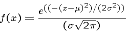
This is centered around the mean, symmetrical, and has tails which go out to infinity in each direction.

The normal distribution is completely parameterized by the mean and standard deviation.

Approximately 2/3 of the probability mass of a normal distribution lies within one standard deviation from the mean.

Approximately 95% of the probability mass of a normal distribution lies within two standard deviations from the mean.

Thus the probability of being far from the mean decreases rapidly - less than one in 10,000 points is more than four two standard deviations from the mean.

What's Normal?

Human heights and weights seem to be fit reasonably well by normal distributions, although the observed distributions do not have tails which go to infinity.

Consider compare this to the distribution of incomes. It is much rarer to find someone twice as tall as the mean than twice as rich as the mean.

The tails of the income distribution go out much further than is supported by a normal distribution.

Stock returns are not completely modeled by normal distributions because:

• a lower bound on return is $-1$, with no upper bound,

• if daily returns were normally distributed, then multiperiod returns are not normal (they would be the product of normals),

• Empirical data suggests that returns show greater kurtosis (fatter tails) than expected with a normal distribution.

The Lognormal Distribution

Another common assumption is that the log returns $r_t$ are normally distributed with mean $\mu$ and variance $\sigma^2$.

Since the sum of a finite number of independent normal random variables is normal, the conceptual problem with multiperiod returns is eliminated

Still, empirical data suggest that returns show greater kurtosis (fatter tails) than expected with a lognormal distribution.

Creating a mixture of two normal distributions with identical mean but different variance can produce fatter tails:

$$r_t \approx (1-\alpha) N(\mu, {\sigma_1}^2) + \alpha N(\mu, {\sigma_2}^2)$$

However, adding parameters requires more data to fit accurately, and are less satisfying theoretically unless you can explain the need for two distributions.

Other distributions, including stable distributions and the Cauchy distribution have been proposed to model returns.

Empirical Properties of Returns

Stock returns exhibit greater kurtosis than the normal or lognormal routines would suggest.

This means that extreme events (both positive and negative) are observed more often than predicted by these distributions.

Stock returns also exhibit a certain amount of skewness. Certainly extreme events are more likely to be crashes than explosions.

figure=figures/ourmodel.eps,width=4in

In general, empirical density functions are taller, skinnier, and have a wider base of support than the corresponding normal density function.