CSE 691 - Lecture 14 - Clustering

Steven S. Skiena

Dept. of Computer Science

SUNY Stony Brook

Similarity Detection in Finance

Many natural problems in finance involve partitioning assets into natural groups or identifying assets with similar properties:

• What company has a balance sheets most similar to Yahoo?

• Which companies have similar patterns of ownership by institutional investors such as mutual funds and pensions?

• Can we partition stocks into logical groups (e.g. by industry) based on time-series and other data?

Building a diversified portfolio is somehow dual to clustering. Diversification means selecting a group of stocks which are as different or uncorrelated as possible.

Distance Measures

Certain mathematical properties are expected of any distance measure, or metric:

1. $d(x,y) \geq 0$ for all $x$, $y$.
2. $d(x,y) = 0$ iff $x=y$.
3. $d(x,y) = d(y,x)$ (symmetry)
4. $d(x,y) \leq d(x,z) + d(z,y)$ for all $x$, $y$, and $z$. (triangle inequality)

Euclidean distance 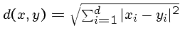$d(x,y) = \sqrt{ \sum_{i=1}^d \vert x_i - y_i\vert^2 }$ is probably the most commonly used metric. Note that it weights all features/dimensions ``equally''.

Variations on Euclidean distance include $L_k$ norms for $k \neq 2$:

$$d(x,y) = (\sum_{i=1}^d \vert x_i - y_i\vert^k )^{(1/k)}$$

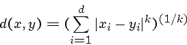
We get the ``Manhattan'' distance metric for $k=1$ and the ``maximum'' component for $k=\infty$.

The correlation coefficient of sequences $X$ and $Y$, yield a number from -1 to 1 but is not a metric.

The loss of the triangle inequality in non-metrics can cause strange clustering behavior, particularly in single linkage methods.

Cluster Analysis

Clustering is an inherently ill-defined problem since the correct clusters depend upon context and are in the eye of the beholder.

figure=figures/where-clusters.eps,width=3.0in

How many clusters are there?

Clustering is an important statistical technique in all experimental sciences, including biology.

Clustering can provide more robust comparisons than pairwise correlation: ``Historically, the single best predictor of the Standard & Poor's 500-stock index was butter production in Bangladesh.''

Agglomerative Clustering

Agglomerative clustering methods merge smaller clusters into bigger clusters incrementally:

figure=figures/dendogram.eps,width=4in

However, there are several ways to measure the distance between two clusters:

figure=figures/single.eps,width=2in figure=figures/centroid.eps,width=2in

figure=figures/average.eps,width=2in figure=figures/complete.eps,width=2in

The choice of measure implies a tradeoff between computational efficiency and robustness.

The simplest merging criteria is to join the two nearest clusters. Minimum spanning tree methods define single-link clustering.

figure=figures/minimum-spanning-tree-L.eps,width=2in figure=figures/minimum-spanning-tree-R.eps,width=2in

In complete link clustering, we merge the pair which minimizes the maximum distance between elements. This is more expensive ($O(n^3)$ vs. $O(n^2)$), but presumably more robust.

$k$-Means Clustering

$k$-Means clustering is an iterative clustering technique where you specify the number of clusters $k$ in advance.

Pick $k$ points, and assign each example to the closest of the $k$ points.

Pick the `average' or `center' point from each cluster, and repeat until sufficiently stable.

Note that such center points are not well defined in clustering non-numerical attributes, such as color, profession, favorite type of music, etc.

The question of how many clusters you have (or expect) is inherently fuzzy in most applications. However, the ``right'' number of clusters, adding another cluster should not dramatically reduce distance from the centers.

Such techniques represent a partitioning-based strategy, which is dual to the notion of agglomerative clustering.

Graph-Theoretic Clustering Methods

An alternate approach to clustering constructs an underlying similarity graph, where elements $i$ and $j$ are connected by an edge iff $i$ and $j$ are similar enough that they should/can be in the same cluster.

If the similarity measure is totally correct and consistent, the graph will consist of disjoint cliques, one per cluster.

figure=figures/clique-L.eps,width=2in figure=figures/clique-R.eps,width=2in

Overcoming spurious similarities reduces to finding maximum-sized cliques, an NP-complete problem.

Overcoming occasional missing edges means we really seek to find sets of vertices inducing dense graphs.

Repeatedly deleting low-degree vertices gives an efficient algorithm for finding an induced subgraph with minimum degree $k$, if one exists.

Cut-Based Algorithms

A real cluster in such a graph should be easy to disconnect by deleting a small number of edges. The minimum edge cut problem asks for the smallest number of edges whose deletion will disconnect the graph.

figure=figures/edge-vertex-connectivity-L.eps,width=2in figure=figures/edge-vertex-connectivity-R.eps,width=2in

The max flow / min cut theorem states that the maximum possible flow between vertices $i$ and $j$ in a weighted graph $G$ is the same as the minimum total edge weight needed to separate $i$ from $j$. Thus network flow can be used to find the minimum cut efficiently.

figure=figures/network-flow-L.eps,width=2in figure=figures/network-flow-R.eps,width=2in

However the globally minimum cut is likely to just slice off a single vertex as opposed to an entire cluster.

Graph Partitioning Approaches

Graph partitioning problems which seek to ensure large components on either side of the cut tend to be NP-complete.

By complementing graph $G$, we get a graph $G'$ with an edge $(i,j)$ in $G'$ iff the edge did not exist in $G$.

By finding the maximum cut in $G'$ and recurring on each side, we can have a top-down (i.e. divisive) clustering algorithm.

figure=figures/max-cut-L.eps,width=2in figure=figures/max-cut-R.eps,width=2in

Finding the maximum cut is NP-complete, but an embarrassingly simple algorithm gives us a cut which is on average half as big as the optimal cut:

For each vertex, flip a coin to decide which side of the cut (left or right) it goes. This means that edge $(i,j)$ has a 50% chance of being cut (yes if coins $i$ and $j$ both came up either heads or tails).

Local improvement heuristics can be used to refine this meaningless cut.

Nearest Neighbor Clustering

Assign each point to its nearest neighbor who has been clustered if the distance is sufficiently small.

Repeat until there are sufficient number of clusters.

Nearest neighbor classifiers assign an unknown sample the classification associated with the closest point.

figure=figures/voronoi-diagrams-R.eps,width=4in

Conceptually, all classifiers carve up space into labeled regions. Voronoi diagrams partition space into cells defining the boundaries of the nearest neighbor regions.

Nearest neighbor classifiers are simple and reasonable, but not robust. A natural extension assigns the majority classification of the $k$ closest points.

figure=figures/overfit.eps,width=4in

An important task in building classifiers is avoiding over-fitting, training your classifier to replicate your data too faithfully.

Other classifier techniques include decision trees and support-vector machines.

Financial Time-Series Clustering: A Case Study

M. Gavrilov, D. Anguelov, P. Indyk, and R. Motwani. Mining the Stock Market: Which Measure is Best?, Proc. Sixth Int. Conf. Knowledge Discovery and Data Mining (KDD), 487-496, 2000.

Their goal was to study different time-series distance measures of stock prices to see which resulted in clusters which best matched standard industrial groups (e.g. semiconductors, aerospace).

They parameterized distance measures by three different dimensions:

• Representation - original time-series or first derivative?

  The first derivative is analogous to returns vs. prices.

• Normalization - do we adjust the time series values to bring all of them to the same scale?

  Global normalization subtracts the series average from each value, and then divides the vector by its L2-norm.

  Piecewise normalization partitions the series into short windows and normalizes on each independently.

• Dimension Reduction - can we reduce the volume of data to analyze by:

  (a) averaging runs of $d$ elements into one,

  (b) Fourier transforming the series and deleting all but low frequencies, or

  (c) using principal components analysis via singular value decomposition to identify the most significant ``dimensions''.

They used Euclidean distance as the similarity measure on the resulting time-series.

They used agglomerative clustering, where they merge the clusters which minimize the maximum distance between two inter-cluster elements.

Results:

The first derivative was much more informative than the original series

Piecewise normalization worked best, with partitioning into 15 day windows.

Dimension reduction via PCA lead to better clusters than the original series.

Difficulties with Clustering

How many clusters should there be? (hint: eyeball it or look for large distances)

How do we visualize large, multidimensional datasets? (hint: read Tufte's books)

How do we handle multidimensional datasets? (hint: dimension reduction techniques such as principle component analysis and singular-value decomposition (SVD))

How do we handle noise? (hint: aim for robustness by avoiding single-linkage methods and proper distance criteria)

Which clustering algorithm should we use? (hint: this probably doesn't make as much difference as you think).

Which distance measure should we use? (hint: this is your most important decision)