Steven S. Skiena
Dept. of Computer Science
SUNY Stony Brook
Fractals are unusual, imperfectly defined, mathematical objects that observe self-similarity, that the parts are somehow self-similar to the whole.
This self-similarity process implies that fractals are scale-invariant, you cannot distinguish a small part from the larger structure, e.g. a tree branching process.
Fractals are interesting because (1) many phenomena in nature are self-similar and scale invariant, and (2) traditional mathematics/geometry does not capture the properties of these shapes.
Mandelbrot defines a fractal set as one in which the fractal dimension is strictly greater than the topological dimension.
The Hurst exponent in R/S analysis is somewhat akin to a fractal dimension.
As has been discussed previously, real financial returns are not accurately modeled by a normal distribution, because there is too much mass at the tails.
In other words, outlying events occur much more frequently in financial returns than they should if normally distributed.
We would expect that the standard deviation of returns should grow at a rate
![]() , where
, where ![]() is the amount of time, if they were normally distributed.
is the amount of time, if they were normally distributed.
In fact, for historical periods on the Dow Jones
up to about
![]() days, the standard deviation grows faster
(0.53), and then drops dramatically (0.25).
days, the standard deviation grows faster
(0.53), and then drops dramatically (0.25).
Thus risk does increase with holding period up to a point, but then favors long-term investors.
We seek distributions which model such phenomenon better.
It is fairly easy to observe the difference between the real distributions of returns and the normal distribution.
It is fairly easy to construct distributions which fit observed data better than normal.
However, what tends to be lacking is an explanation of how the distribution arises.
The Fractal Market Hypothesis (Peters, 1994) states:
A central tool of fractal data modeling is rescaled range or R/S analysis.
We have seen how
unbiased coin flipping leads to the
the expected the difference between the number of heads and tails in an
![]() tosses of an unbiased coin is
tosses of an unbiased coin is
![]() .
.
This is characteristic of random walk models and Brownian motion, that
![]() , where
, where ![]() is the distance traveled,
is the distance traveled, ![]() is time,
is time, ![]() is a
constant and
is a
constant and ![]() is the exponent.
is the exponent.
How could we discover this exponent ![]() experimentally, for say, a run of coin
flipping?
We could build up time series
experimentally, for say, a run of coin
flipping?
We could build up time series
![]() , where
, where ![]() if
the
if
the ![]() th flip heads and
th flip heads and ![]() if the
if the ![]() th flip is tails.
th flip is tails.
By taking the log of both sides of the equation,
Thus by doing a linear regression on the log scaled distance and time series
we will discover ![]() and, more importantly,
and, more importantly, ![]() .
.
In any process modeled by an unbiased random walk, ![]() .
.
A hydrologist studying floods, H. E. Hurst, did similar analysis on 847 years worth
of data on overflows of the Nile River, and found an exponent ![]() .
.
This implies that the accumulated deviation from expectation was growing much faster than expected from an unbiased random walk of independent observations.
Another way to think about this is that extreme events (e.g. long runs of heads/tails, or heavy floods) were more common than
It implied that the individual observations where not really independent - although they were not accurately modeled by a simple autoregressive process.
Hurst did a similar analysis of many different processes, including rainfall,
temperature, and sunspot data, and consistently got ![]() .
This quantity
.
This quantity ![]() is now called the Hurst exponent.
is now called the Hurst exponent.
A Hurst exponent of ![]() implies an independent process.
It does require that it be Gaussian, just independent.
R/S analysis is non-parametric, meaning there is no assumption / requirement
of the shape of the underlying distribution.
implies an independent process.
It does require that it be Gaussian, just independent.
R/S analysis is non-parametric, meaning there is no assumption / requirement
of the shape of the underlying distribution.
Hurst exponents of ![]() imply a persistent time series characterized
by long memory effects.
imply a persistent time series characterized
by long memory effects.
Hurst exponents of
![]() imply an anti-persistent time series,
which covers less distance than a random process.
Such behavior is observed in mean-reverting processes, although that assumes
that the process has a stable mean.
imply an anti-persistent time series,
which covers less distance than a random process.
Such behavior is observed in mean-reverting processes, although that assumes
that the process has a stable mean.
Given a time sequence of observations ![]() , define the series
, define the series
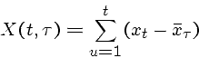
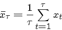
Thus ![]() measures difference sum of the observations time 1 to
measures difference sum of the observations time 1 to ![]() compared to the average of the first
compared to the average of the first ![]() observations.
observations.
The self-adjusted range ![]() is defined
is defined
The standard deviation as a function ![]() is
is
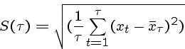
Finally, the self-rescaled, self adjusted range is
Basically, it compares the largest amount of change happens over the
initial ![]() terms to what would be expected given their variance.
terms to what would be expected given their variance.
The asymptotic behavior of ![]() is
provably
is
provably
In plotting
![]() against
against ![]() , we expect to get
a line whose slope determines the Hurst exponent.
, we expect to get
a line whose slope determines the Hurst exponent.
In practice for financial data, this line fits a straight line
up to some ![]() , and then breaks down.
, and then breaks down.
This ![]() gives some idea of a cycle time, over which there is dependence
upon the past.
gives some idea of a cycle time, over which there is dependence
upon the past.
Mandelbrot proposed a multi-fractal generating process to generate time-series which have the persistence effects resembling financial time series:
Another process which yields burstier walks than coin-flipping states
that we will repeat the previous step (up or down) with probability ![]() and reverse with probability
and reverse with probability ![]() .
.
If ![]() this is just coin flipping, but other exponents/probabilities
yield interesting walks.
this is just coin flipping, but other exponents/probabilities
yield interesting walks.
We found that ![]() matched price behavior better than
matched price behavior better than ![]() .
.
Consider the following betting strategy.
Buy a stock now.
Sell it when it gets up to price ![]() , or drops down to price
, or drops down to price ![]() .
.
For ![]() , is there a strategy (i.e.
, is there a strategy (i.e. ![]() ,
, ![]() pair) which will return an expected
profit (e.g. 10, 100)?
The answer is no - why?
pair) which will return an expected
profit (e.g. 10, 100)?
The answer is no - why?
What about ![]() ?
The answer is yes - why?
?
The answer is yes - why?
Is this a winning idea? Only if (1) prices really are modeled by Hurst walks, (2) transaction costs are insignificant, (3) there is not an upward trend where buy and hold becomes more profitable...