Steven S. Skiena
Dept. of Computer Science
SUNY Stony Brook
In the fixed fluctuation model, all returns are either ![]() or
or
![]() .
.
Such a model is consistent with our random walk model, although we picture the return sequences as being generated by a hostile rather than random adversary.
It can also be thought of time scaling model, where we consider
each return of ![]() or
or ![]() as one step, regardless of how
long it took to take that step.
as one step, regardless of how
long it took to take that step.
An ![]() -adversary generates length-
-adversary generates length-![]() binary sequences on
binary sequences on
![]() where exactly
where exactly ![]() individual returns are profitable.
individual returns are profitable.
Thus the optimal offline return is ![]() .
.
Let ![]() denote the optimal money making algorithm against this adversary
and
denote the optimal money making algorithm against this adversary
and ![]() be its return.
Then:
be its return.
Then:
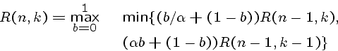
It can be proven that ![]() is always better than optimal
offline buy and hold.
is always better than optimal
offline buy and hold.
For the constant rebalancing strategy ![]() ,
the optimal rebalancing constant
,
the optimal rebalancing constant
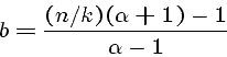
This constant rebalancing strategy is also better than buy and hold - however we assume no transaction costs.
The downside of ![]() and other provably money making algorithms is that
they cannot invest much money in the earlier periods of the game,
which limits total returns.
and other provably money making algorithms is that
they cannot invest much money in the earlier periods of the game,
which limits total returns.
This kind of recurrence gives rise to a graph of possible paths called a binomial tree within the finance literature:
Binomial trees are used compute option prices in a similar manner as we are using them.
We assume that there is given probability
of upward ![]() and downward
and downward ![]() moves.
moves.
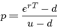
We can use an arbitrage argument to set the probability ![]() as a function
of the risk-free rate.
as a function
of the risk-free rate.
At any point, investors can either (a) hold stock or (b) invest at the
risk-free rate ![]() .
.
A risk-neutral investor would not care which portfolio they owned if they had the same return.
Setting equal the returns from the stock (
![]() )
and the risk-free portfolio (
)
and the risk-free portfolio (![]() ), we can solve for
), we can solve for ![]() to determine
the risk-neutral probability.
to determine
the risk-neutral probability.
In truth, investors are not risk-neutral. In order to take the riskier investment they must be paid a premium.
Binomial trees are used to price option using the idea of risk-neutral valuation.
Suppose a stock price is currently at $20, and will either be at $22 or $18 in three months.
What is the price of a European call option for a strike price of $21? Clearly, this reduces to determining the probability of the upward price movement.
The risk-neutral investor argument for setting this probability can be applied if we set up two portfolios which are of provably of equal risk.
We will construct two riskless portfolios, one involving the stock and the other the risk-free rate.
A riskless portfolio can be created by buying ![]() shares of stock
and selling a short position in 1 call option, such that the value of the
portfolio is the same whether the stock moves up or down.
shares of stock
and selling a short position in 1 call option, such that the value of the
portfolio is the same whether the stock moves up or down.
If the stock moves to $22, our portfolio will
be worth
![]() ,
since we must pay the return of the option we sold.
,
since we must pay the return of the option we sold.
If the stock moves to $18, our portfolio will be worth
![]() ,
since the option we sold is worthless.
,
since the option we sold is worthless.
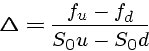
A riskless portfolio is constructed by buying ![]() shares,
since it is the solution of
shares,
since it is the solution of
![]() .
.
Whether the stock goes up or down, this portfolio is worth ![]() at the end of the period.
at the end of the period.
The discounted value of this portfolio today, ![]() , can be computed given the
risk-free interest rate
, can be computed given the
risk-free interest rate ![]() .
.
Since the value of ![]() is equal to owning
is equal to owning ![]() shares of stock
at $20 per share minus the value
shares of stock
at $20 per share minus the value ![]() of the option,
of the option,
![]() .
.
In general, if there is an upward price movement, the value at the end
of the option is
If there is a downward rice movement, the value at the end
of the option is
Setting them equal and solving for ![]() yields
yields
The present value of the portfolio with a risk-free rate of ![]() is
is
Equating these two and solving for ![]() yields
yields
By definition, the value of ![]() must also be
must also be
Solving for ![]() we get
we get
Binomial trees are widely used to price options.
Adding additional levels to the trees allows finer price gradations than just a single up or down.
The value of the option can be worked backwards from the terminating (basis) condition level by level.
The value of the option on terminating level is clear since the stock price determined.
The price of an option generally converges for about ![]() levels
levels
This binomial tree model can be generalized to include the effects of (1) dividends, by changing the magnitude of the moves in the levels corresponding to dividend periods, (2) changing interest rates, by using the rate appropriate on a given yield curve.
It can also be generalized to allow more than two price movements from each node, say increase, decrease, and unchanged.
Once the number of levels gets too high for exhaustive computation, we can use Monte Carlo random walks to price the option.
Note that the number of options needed (![]() )
changes at each node/level in the binomial tree.
Thus to maintain a riskless portfolio options must be bought and
sold continuously, a process known as delta hedging.
)
changes at each node/level in the binomial tree.
Thus to maintain a riskless portfolio options must be bought and
sold continuously, a process known as delta hedging.