


In our challenge, we have to predict the age at which given celebrity will die. Since the output variable is not class labels, this is not a classification problem. Here the output variable Age at which celebrity will die is continuous value which is clearly regression problem. So we have referred many papers to understand how Age can be used as output variable in various Machine learning regression models.
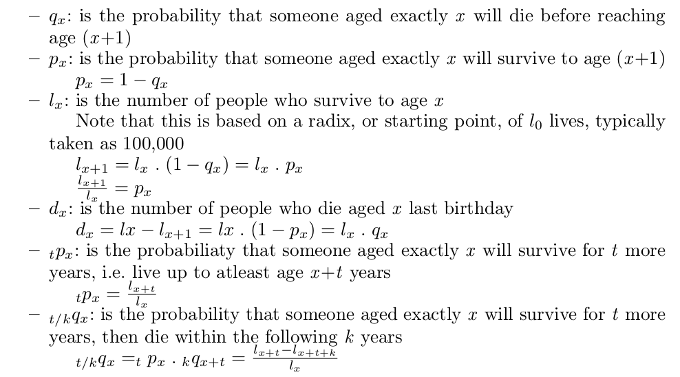
 where dx is the number of deaths occurring between ages x and x+1, and Lx is the number of person-years lived by the life table cohort between ages x and x+1. The conversion of the age-specific death rate, mx to the age-specific probability of death qx(formula) is as follows:

Initially we had explored various sources for gathering our data. Like the Notable Names Database, Wikipedia, DBpedia and Freebase. Notable Names Database (NNDB) consists of data of more than 40,000 very famous people. But this was too small for our needs. We considered parsing Wikipedia, but due to its unstructured nature, even a robust web crawler was failing to get all the information we need easily. This led us to DBpedia. It exposes Wikipedia has a structured database. This seemed good for our needs before we explored Free- base. Freebase is a community-curated database of well-known people, places, and things. Freebase consists of data from Wikipedia as well as some other sources, for example, biographies of people. The persons in Wikipedia is subset of the ones in Freebase. Using Freebase effectively increases our dataset size and hence we finalized on using it for our dataset.
For the life tables our possible data sources were the World Health Orga- nization (WHO) life tables and the Social Security Agency (SSA) actuarial life tables. We have compared the two in the "Evaluation of Life Tables" section and justified our decision to use the SSA actuarial life tables for the life expectancy predictions.
Freebase classifies objects using ontology. We are interested only in famous people. The persons class is useful in our case. Freebase has information of more than 2 million people. It was recently bought over by Google and we use Google APIs for Freebase to collect information from it.
Along with the APIs we use the Meta-web Query Language (MQL) for Free- base to query the Data we need. MQL is similar the Structured Query Language (SQL) to filter queries to return only the data that is necessary.
Figure below shows a block diagram of the information extractor we developed to gather our dataset. First we use MQL to make a query for all unique persons. We use the APIs to send this request and it returns to us unique IDs for about 1000 people at a time. We use an iterator to get 1000 IDs at a time until we have all the IDs. We collected 2,274,435 IDs. We then send a request to get information about each person using the person’s ID, one by one. We get fields like Name, Date of Birth, Date of Death (if dead), Age, Gender, Nationality, Cause of death, Profession, etc. Freebase imposes a limit of 100K queries per user per day, hence we used multiple user accounts over 2 weeks to collect information about each person.
We have a dataset of 2,274,435 rows (people) in total. We have collected many fields (columns) for each person. In total our dataset has 63 columns. Some of them are Name, Date of Birth, Date of Death, Age, Birth Place, Nationality, Gender, Cause of death, Profession(s), Religion, Ethnicity, Spouse/Partner, Education, etc. Clearly, not all fields are relevant for models currently, but since we had almost no extra cost in collecting them we have included them. This will help us in our next steps in case we find interesting ways to use them in our models. We remove the (currently) irrelevant columns in the data filtering phase.
We first did some basic cleaning on this dataset. We have deleted rows that do not contain a date of birth for a person. We have used one main profession for people who were classified into many professions. We also performed some other minor cleaning up like removing null rows and random strings in numeric columns.
Next we had to do a lot of preprocessing on our dataset before it can be used on our machine learning models.
Firstly, we needed a way to specify the profession a person belongs to numerically. For this, we made a new column for each profession that we are interested in modeling and marked a 1 there if the person belongs to that profession and a 0 if he/she does not.
Secondly, we needed a way to specify the nationality of a person numerically. For this we hashed each country to a unique numeric ID and created a new column for each person identifying the nationality id he/she belongs to.
Third, we needed a way to specify the gender numerically. We used 0 to represent a male and 1 in case of a female.
Fourth, we decided to use the dead people in our dataset for training purposes. Hence, we filtered to include only dead people. The 2010 life tables would not depict good predictions for persons born very early in the timeline, say in 1800. Hence we further filtered to include dead people born only after the year 1890.
Finally and most importantly. After seeing incorrect results from models that predict the year a person would die and/or the age he/she would die and after discussing the same with Professor Skiena[7]. We decided to manipulate our dataset in a way that we can predict the number of remaining years in a person’s life. For this we took 4 different years into consideration, namely, 1915, 1940, 1965 and 1990. For each person we calculate the remaining years from each of the aforementioned years. Thus we have the current age of the person at the year under consideration and the number of more years the person lived from his/her current age. Our code is robust enough to do this process for more than the 4 years taken into consideration, if necessary. This process effectively increases the size of our dataset by 4 times.
We are quite satisfied with our data set, we have used an apt source given our project domain and the data set is large enough for us to sample and develop machine learning based models.
We have heavily modularized our development and evaluation environment. Figure below shows a block diagram of the same. Basically we just run a single command, which trains and tests our data and generate statistics of each model we have implemented and also tells which one is performing the best based on these statistics.
Figure 4: Development Environment
After the steps taken on our dataset described in the previous section we divided our data into train and test parts. We have used 80% of our data for training and 20% as test data for evaluation. After this we pass the training and test data as parameters to one of the many machine learning algorithms we use which we describe in the next section. Once the training is done, we generate a summary, which consists of the coefficients assigned by the machine learning algorithm and statistics about the training.
We then evaluate the model on our test data and the stats function then generates statistics about the evaluation. It compares the test data predictions of remaining years of a person’s life to the actual remaining years the person had. The evaluation statics we report are:
The stats() function also generates a scatter plot comparing the actual and predicted values. The stats() function also generates an error plot for the error made in the predictions. Then another function uses this model to make predictions of remaining years on our final dataset (of the 32 persons given by Prof. Skiena).
In this section we will explain our baseline model
Initially, we used WHO life tables for our baseline model but now we are now using the SSA actuarial life tables instead of the WHO tables. We also make predictions on the remaining life a person has rather than the probability of death of the person.
The reason for the same is presented in the life table evaluations section further.
The baseline model basically gets the expected remaining life span of a person from the life tables given the persons age and gender. We evaluated our baseline model. Figure shows the evaluation statistics.
We used Liner Regression (also called Ordinary Least Squares, a type of supervised learning method) on our dataset. Linear Regression fits a linear model with coefficients w = (w 1, ..., w p) to minimize the residual sum of squares between the observed responses in the dataset, and the responses predicted by the linear approximation.
We used Ridge Regression on our dataset. It addresses some of the problems of Ordinary Least Squares by imposing a penalty on the size of coefficients. Here, α ≥ 0 is a complexity parameter that controls the amount of shrinkage: the larger the value of α, the greater the amount of shrinkage and thus the coefficients become more robust to collinearity. We have selected an α value of 1.
Neighbors-based regression can be used in cases where the data labels are continuous rather than discrete variables. The label assigned to a query point is computed based on the mean of the labels of its nearest neighbors. The basic Nearest Neighbors Regression uses uniform weights that is, each point in the local neighborhood contributes uniformly to the classification of a query point.
Under some circumstances, it can be advantageous to weight points such that nearby points contribute more to the regression than faraway points. This can be accomplished through the weights keyword. The default value, weights = ’uniform’, assigns equal weights to all points. weights = ’distance’ assigns weights proportional to the inverse of the distance from the query point. Alternatively, a user-defined function of the distance can be supplied, which will be used to compute the weights.
We found k=10 to be the optimal value during our testing.
Decision Trees (DTs) are a non-parametric supervised learning method used for classification and regression. The goal is to create a model that predicts the value of a target variable by learning simple decision rules inferred from the data features.
A random forest is a meta estimator that fits a number of classifying decision trees on various sub-samples of the dataset and use averaging to improve the predictive accuracy and control over-fitting.
In total, we evaluated 6 machine learning algorithms. Figure below shows the evaluation statistics for all the machine learning models. Figure below also summarizes the performance of each of these algorithms and highlights the best one, based on the Mean Absolute Error (MAE). Ridge Regression performed the best .
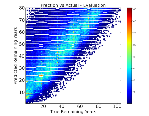
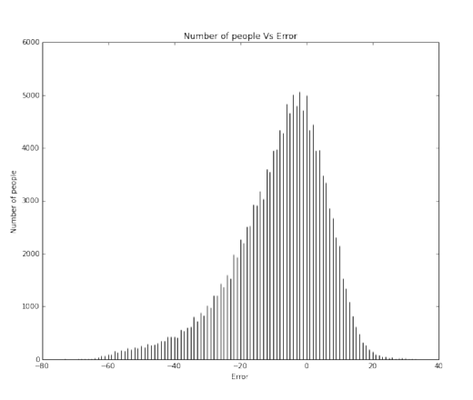
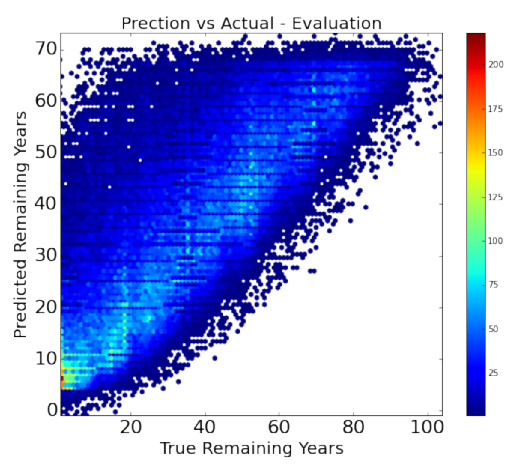
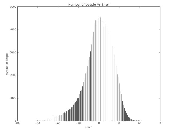
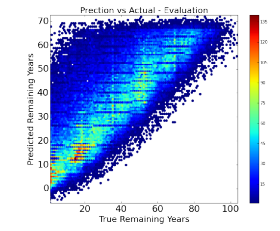
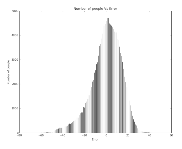
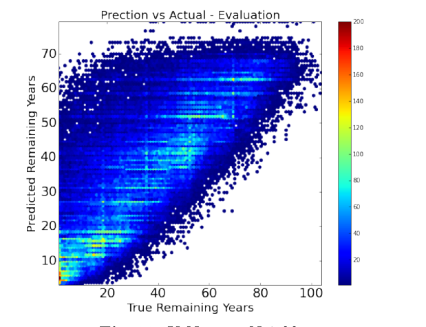

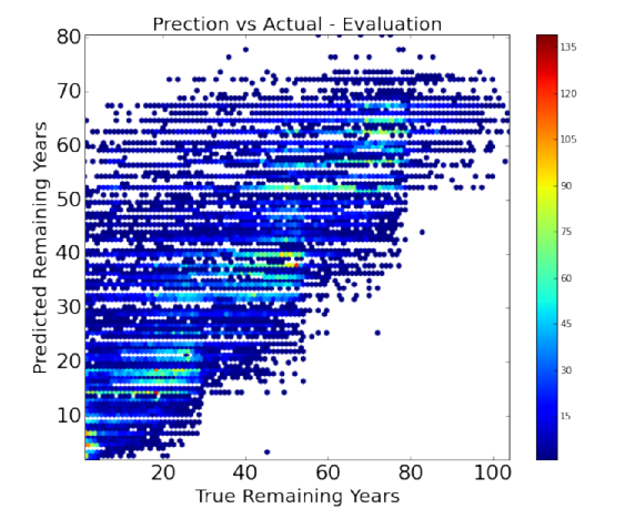

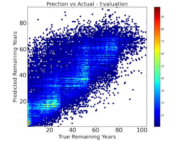
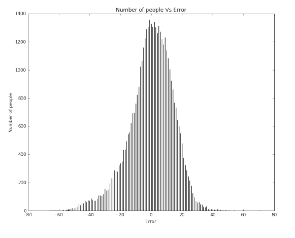
It is clear to us that overall our models are better than the baseline (if at all) by a very small margin. Our models achieved a maximum of about 12% better than the baseline model for ridge regression. We understand that we need to significantly improve our models to give a much better efficiency.
Ridge Regression is currently the best model. The current predictions as per the ridge regression are shown in the left figure.
These predictions do look good to us for a few reasons.
Firstly, we observe that Rock/Music star and to some extent Movie stars are penalized by the model, predicting they would have shorter lives than others.
Secondly, Scientists are observed to live a little longer than others as observed with Stephen Hawking.