Which Digit?
|
Which Digit? |
In this project, you will design two classifiers: a naive Bayes classifier and Decision tree classifier. You will test your classifiers on a image data set: a set of scanned handwritten digit images. Even with simple features, your classifiers will be able to do quite well on these tasks when given enough training data.
Optical character recognition (OCR) is the task of extracting text from image sources. The first data set on which you will run your classifiers is a collection of handwritten numerical digits (0-9). This is a very commercially useful technology, similar to the technique used by the US post office to route mail by zip codes.
The code for this project includes the following files and data, available as a zip file.
Data file |
|
data.zip |
Data file, including the digit and face data. |
Files you will edit |
|
naiveBayes.py |
The location where you will write your naive Bayes classifier. |
id3.py |
The location where you will write your ID3 (Decision Tree) classifier. |
dataClassifier.py |
The wrapper code that will call your classifiers. You will also write your enhanced feature extractor here. You will also use this code to analyze the behavior of your classifier. |
answers.py |
Answers to Question 3 go here. |
Files you should read but NOT edit |
|
classificationMethod.py |
Abstract super class for the classifiers you will write. (You should read this file carefully to see how the infrastructure is set up.) |
samples.py |
I/O code to read in the classification data. |
util.py |
Code defining some useful tools. You may be familiar with some of these by now, and they will save you a lot of time. |
mostFrequent.py |
A simple baseline classifier that just labels every instance as the most frequent class. |
What to submit: You will fill in portions of naiveBayes.py,dataClassifier.py and answers.py
(only) during the assignment, also you need to write the whole class for Decision Tree classifier in id3.py and submit them.
Academic Dishonesty: We will be checking your code against other submissions in the class for logical redundancy. If you copy someone else's code and submit it with minor changes, we will know. These cheat detectors are quite hard to fool, so please don't try. We trust you all to submit your own work only; please don't let us down. Instead, contact the course staff if you are having trouble.
To try out the classification pipeline, run dataClassifier.py
from the command line. This
will classify the digit data using the default classifier (mostFrequent) which blindly classifies every example
with the most frequent label.
python dataClassifier.py
As usual, you can learn more about the possible command line options by running:
python dataClassifier.py -h
We have defined some simple features for you.
Later you will design some better features. Our simple feature set includes one feature for
each pixel location, which can take values 0 or 1 (off or on). The features are encoded as
a Counter where keys are feature locations (represented as (column,row)) and
values are 0 or 1.
Implementation Note: You'll find it easiest to hard-code the binary feature assumption. If you do, make sure you don't include any non-binary features. Or, you can write your code more generally, to handle arbitrary feature values, though this will probably involve a preliminary pass through the training set to find all possible feature values (and you'll need an "unknown" option in case you encounter a value in the test data you never saw during training).
id3.py. For initial debugging, it is recommended that you construct a very simple data set (e.g., based on a boolean formula) and test your program on it. A skeleton implementation of a naive Bayes classifier is provided for you in
naiveBayes.py.
You will fill in the trainAndTune function, the
calculateLogJointProbabilities function and the
findHighOddsFeatures function.
A naive Bayes classifier
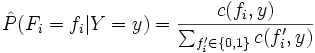
models a joint distribution over a label ![]() and a set of observed random variables, or features,
and a set of observed random variables, or features,
![]() ,
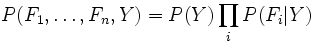
using the assumption that the full joint distribution can be factored
as follows (features are conditionally independent given the label):
,
using the assumption that the full joint distribution can be factored
as follows (features are conditionally independent given the label):
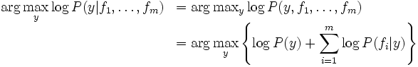
To classify a datum, we can find the most probable label given the feature values for each pixel, using Bayes theorem:
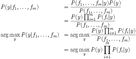
Because multiplying many probabilities together often results in underflow, we will instead compute log probabilities which have the same argmax:
To compute logarithms, use math.log(), a built-in Python function.
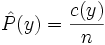
We can estimate ![]() directly from the training data:
directly from the training data:
The other parameters to estimate are the conditional probabilities of
our features given each label y:
![]() . We do this for each
possible feature value (
. We do this for each
possible feature value (![]() ).
).
In this project, we use Laplace smoothing, which adds k counts to every possible observation value:
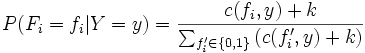
If k=0, the probabilities are unsmoothed. As k grows larger, the probabilities are smoothed more and more. You can use your validation set to determine a good value for k. Note: don't smooth P(Y).
Question 2 (50 points)
Implement trainAndTune and calculateLogJointProbabilities in naiveBayes.py.
In trainAndTune, estimate conditional probabilities from the training data for each possible value
of k given in the list kgrid.
Evaluate accuracy on the held-out validation set for each k and choose
the value with the highest validation accuracy. In case of ties,
prefer the lowest value of k. Test your classifier with:
python dataClassifier.py -c naiveBayes --autotune
Hints and observations:
calculateLogJointProbabilities uses the conditional probability tables constructed by
trainAndTune to compute the log posterior probability for
each label y given a feature vector. The comments of the method describe
the data structures of the input and output.
analysis method in dataClassifier.py to explore the mistakes that your classifier is making. This is optional.
--autotune option. This will ensure that kgrid has only one value, which you can change with -k.
--autotune, which tries different values of k, you should get a validation accuracy of about 74% and a test accuracy of 65%.
Counter.argMax() method.
-d faces (optional).
Another, better, tool for understanding the parameters is to look at odds ratios. For each pixel
feature ![]() and classes
and classes ![]() , consider the odds ratio:
, consider the odds ratio:
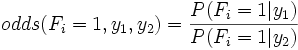
The features that have the greatest impact at classification time are those with both a high probability (because they appear often in the data) and a high odds ratio (because they strongly bias one label versus another).
Question 3 (EXTRA 10 points)
Fill in the function findHighOddsFeatures(self, label1, label2).
It should return a list of the 100 features with highest odds ratios for label1
over label2.
The option -o activates an odds ratio analysis.
Use the options -1 label1 -2 label2 to specify which labels
to compare. Running the following command will show you the 100 pixels
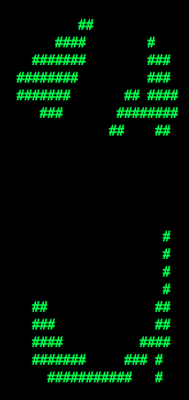
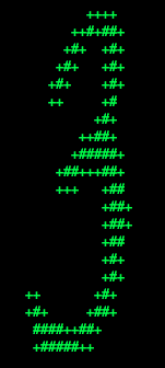
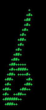
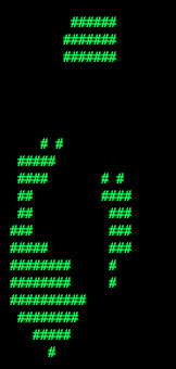
that best distinguish between a 3 and a 6.
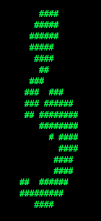
python dataClassifier.py -a -d digits -c naiveBayes -o -1 3 -2 6Use what you learn from running this command to answer the following question. Which of the following images best shows those pixels which have a high odds ratio with respect to 3 over 6? (That is, which of these is most like the output from the command you just ran?)
 |
 |
 |
 |
 |
q2 in answers.py.
Building classifiers is only a small part of getting a good system working for a task. Indeed, the main difference between a good classification system and a bad one is usually not the classifier itself (e.g. decision tree vs. naive Bayes), but rather the quality of the features used. So far, we have used the simplest possible features: the identity of each pixel (being on/off).
To increase your classifier's accuracy further, you will need to extract
more useful features from the data. The EnhancedFeatureExtractorDigit
in dataClassifier.py
is your new playground. When analyzing your classifiers' results, you
should look at some of your errors and look for characteristics of the
input that would
give the classifier useful information about the label. You can add
code to the analysis function in dataClassifier.py
to inspect what your classifier is doing.
For instance in the digit data, consider the number of
separate, connected regions of white pixels, which varies by digit type.
1, 2, 3, 5, 7 tend to have one
contiguous region of white space while the loops in 6, 8, 9 create more.
The number of white regions in a
4 depends on the writer. This is an example of a feature that is not
directly
available to the classifier from the per-pixel information. If your
feature
extractor adds new features that encode these properties,
the classifier will be able exploit them. Note that some features may
require non-trivial computation to extract, so write efficient and
correct code.
Question 4 (EXTRA 10 points)
Add new features for the digit dataset in the
EnhancedFeatureExtractorDigit function in such a way that it works
with your implementation of the naive Bayes classifier: this means that
for this part, you are restricted to features which can take a finite number of discrete
values (and if you have assumed that features are binary valued, then you are restricted to binary features).
Note that you can encode a feature which takes 3 values [1,2,3] by using 3
binary features, of which only one is on at the time, to indicate which
of the three possibilities you have. In theory, features aren't conditionally independent as naive Bayes requires,
but your classifier can still work well in practice. We will test your classifier with the following command:
python dataClassifier.py -d digits -c naiveBayes -f -a -t 1000With the basic features (without the
-f option), your optimal
choice of smoothing parameter should yield 82% on the validation set with a
test performance of 79%. You will receive 3 points for implementing new feature(s)
which yield any improvement at all. You will receive 3 additional points if your new feature(s) give you a
test performance greater than or equal to 84% with the above command.