Steven S. Skiena
Faster than O( ![]() ) Sorting?
) Sorting?
Can we find a sorting algorithm which does significantly better than comparing each pair of elements? If not, we are doomed to quadratic time complexity....
Since sorting large numbers of items is such an important
problem - an ![]() algorithm is the way to go!
algorithm is the way to go!
Logarithms
It is important to understand deep in your bones what logarithms are and where they come from.
A logarithm is simply an inverse exponential function.
Saying ![]() is equivalent to saying that
is equivalent to saying that ![]() .
.
Exponential functions, like the amount owed on a n year
mortgage at an interest rate of ![]() per year, are functions which grow distressingly fast.
Thus inverse exponential functions, ie. logarithms, grow refreshingly slowly.
per year, are functions which grow distressingly fast.
Thus inverse exponential functions, ie. logarithms, grow refreshingly slowly.
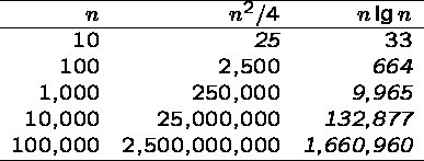
Binary search is an example of an ![]() algorithm.
After each comparison, we can throw away half the possible number of keys.
Thus twenty comparisons suffice to find any name in the million-name Manhattan
phone book!
algorithm.
After each comparison, we can throw away half the possible number of keys.
Thus twenty comparisons suffice to find any name in the million-name Manhattan
phone book!
If you have an algorithm which runs in ![]() time, take it,
because this is blindingly
fast even on very large instances.
time, take it,
because this is blindingly
fast even on very large instances.
Properties of Logarithms
Recall the definition, ![]() .
.
Asymptotically, the base of the log does not matter:
![]()
Thus, ![]() ,
and note that
,
and note that ![]() is just a constant.
is just a constant.
Asymptotically, any polynomial function of n does not matter:Note that
![]()
since ![]() , and
, and
![]() .
.
Any exponential dominates every polynomial. This is why we will seek to avoid exponential time algorithms.
Federal Sentencing Guidelines
2F1.1. Fraud and Deceit; Forgery; Offenses Involving Altered or Counterfeit Instruments other than Counterfeit Bearer Obligations of the United States.
(a) Base offense Level: 6
(b) Specific offense Characteristics
(1) If the loss exceeded $2,000, increase the offense level as follows:
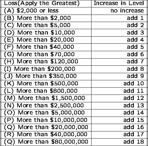
The federal sentencing guidelines are designed to help judges be consistent in assigning punishment. The time-to-serve is a roughly linear function of the total level.
However, notice that the increase in level as a function of the amount of money you steal grows logarithmically in the amount of money stolen.
This very slow growth means it pays to commit one crime stealing a lot of money, rather than many small crimes adding up to the same amount of money, because the time to serve if you get caught is much less.
The Moral: ``if you are gonna do the crime, make it worth the time!''
Mergesort
Given two sorted lists with a total of n elements, at most n-1 comparisons are required to merge them into one sorted list. Repeatedly compare the top elements on each list.
Example: ![]() and
and ![]() .
.
No more comparisons are needed once the list is empty.
Fine, but how do we get the smaller sorted lists to start with? We do merges of even smaller lists!
Working backwards, we eventually get to lists of one element, which are by definition sorted!
Mergesort Example
![]()
![]()
![]()
![]()
Note that on each iteration, the size of the sorted lists doubles, form 1 to 2 to 4 to 8 to 16 ...to n.
How many doublings (or iterations) does it take before the
entire array of size n is sorted?
Answer: ![]() .
.
How much work do we do per iteration?
In merging the lists of 1 element, we have ![]() merges, each
requiring 1 comparison, for a total of
merges, each
requiring 1 comparison, for a total of ![]() comparisons.
comparisons.
In merging the lists of 2 elements, we have ![]() merges,
each requiring at most 3 comparisons, for a total of
merges,
each requiring at most 3 comparisons, for a total of ![]() comparisons.
comparisons.
...
In merging the lists of 2 elements, we have ![]() merges,
each requiring at most
merges,
each requiring at most ![]() comparisons, for a total of
comparisons, for a total of
![]() .
.
This is always less than n per stage!!!
If we make at most n comparisons in each of ![]() stages, we make
at most
stages, we make
at most ![]() comparisons in total!
comparisons in total!
Make sure you understand why mergesort is ![]() - it is
the conceptually simplest
- it is
the conceptually simplest ![]() algorithm we will see.
algorithm we will see.
Space Requirements for Mergesort
How much extra space (over the space used to represent the input elements) do we need to do mergesort?
It is easy to merge two sorted linked lists without using any extra space.
However, to merge two sorted arrays (or portions of an array), we must use a third array to store the result of the merge. This avoids steping on elements we have not needed yet:
Example: Merge ((4,5,6), (1,2,3)).
QuickSort
Although Mergesort is ![]() , it is somewhat inconvienient to
implementate using arrays, since we need space to merge.
, it is somewhat inconvienient to
implementate using arrays, since we need space to merge.
In practice, the fastest sorting algorithm is Quicksort, which uses partitioning as its main idea.
Example: Pivot about 10.
17 12 6 19 23 8 5 10 - before
6 8 5 10 23 19 12 17 - after
Partitioning places all the elements less than the pivot in the left part of the array, and all elements greater than the pivot in the right part of the array. The pivot fits in the slot between them.
Note that the pivot element ends up in the correct place in the total order!
Partitioning the elements
Once we have selected a pivot element, we can partition the array in one linear scan, by maintaining three sections of the array: < pivot, > pivot, and unexplored.
Example: pivot about 10
| 17   12   6   19   23    8   5  | 10
|  5   12   6   19   23    8 | 17
   5 | 12   6   19   23    8 | 17
   5 | 8    6   19   23 | 12   17
   5   8  | 6   19   23 | 12   17
   5   8    6 | 19   23 | 12   17
   5   8    6 | 23 | 19   12   17
   5   8    6 ||23   19   12   17
   5   8    6   10   19   12   17   23
As we scan from left to right, we move the left bound to the right when the element is less than the pivot, otherwise we swap it with the rightmost unexplored element and move the right bound one step closer to the left.
Since the partitioning step consists of at most n swaps, takes time linear in the number of keys. But what does it buy us?
Thus we can sort the elements to the left of the pivot and the right of the pivot independently!
This gives us a recursive sorting algorithm, since we can use the partitioning approach to sort each subproblem.
Quicksort Implementation
MODULE Quicksort EXPORTS Main;            (*18.07.94. LB*)
(* Read in an array of integers, sort it using the Quicksort algorithm,
   and output the array.

   See Chapter 14 for the explanation of the file handling and Chapter
   15 for exception handling, which is used in this example.
*)

  IMPORT SIO, SF;

  VAR
    out: SIO.Writer;

  TYPE
    ElemType = INTEGER;
  VAR
    array: ARRAY [1 .. 10] OF ElemType;

  PROCEDURE InArray(VAR a: ARRAY OF ElemType) RAISES {SIO.Error} =
  (*Reads a sequence of numbers. Passes SIO.Error for bad file format.*)
  VAR
    in:= SF.OpenRead("vector");           (*open input file*)
  BEGIN
    FOR i:= FIRST(a) TO LAST(a) DO a[i]:= SIO.GetInt(in) END;
  END InArray;

  PROCEDURE OutArray(READONLY a: ARRAY OF ElemType) =
  (*Outputs an array of numbers*)
  BEGIN
    FOR i:= FIRST(a) TO LAST(a) DO SIO.PutInt(a[i], 4, out) END;
    SIO.Nl(out);
  END OutArray;

  PROCEDURE Quicksort(VAR a: ARRAY OF ElemType; left, right: CARDINAL) =
  VAR
    i, j: INTEGER;
    x, w: ElemType;
  BEGIN

   (*Partitioning:*)
    i:= left;                             (*i iterates upwards from left*)
    j:= right;                            (*j iterates down from right*)
    x:= a[(left + right) DIV 2];          (*x is the middle element*)
    REPEAT
      WHILE a[i] < x DO INC(i) END;       (*skip elements < x in left part*)
      WHILE a[j] > x DO DEC(j) END;       (*skip elements > x in right part*)
      IF i <= j THEN
        w:= a[i]; a[i]:= a[j]; a[j]:= w;  (*swap a[i] and a[j]*)
        INC(i);
        DEC(j);
      END; (*IF i <= j*)
    UNTIL i > j;

    (*recursive application of partitioning to subarrays:*)

    IF left < j  THEN Quicksort(a, left, j) END;
    IF i < right THEN Quicksort(a, i, right) END;

  END Quicksort;

BEGIN
  TRY                                         (*grasps bad file format*)
    InArray(array);                           (*read an array in*)
    out:= SF.OpenWrite();                     (*create output file*)
    OutArray(array);                          (*output the array*)
    Quicksort(array, 0, NUMBER(array) - 1);   (*sort the array*)
    OutArray(array);                          (*display the array*)
    SF.CloseWrite(out);                       (*close output file to make it permanent*)
  EXCEPT
    SIO.Error =>  SIO.PutLine("bad file format");
  END; (*TRY*)
END Quicksort.
Best Case for Quicksort
Since each element ultimately ends up in the correct position, the algorithm correctly sorts. But how long does it take?
The best case for divide-and-conquer algorithms comes when we split the input as evenly as possible. Thus in the best case, each subproblem is of size n/2.
The partition step on each subproblem is linear in its size.
Thus the total effort in partitioning the ![]() problems of size
problems of size
![]() is O(n).
is O(n).
The recursion tree for the best case looks like this:
The total partitioning on each level is O(n),
and it take ![]() levels of perfect partitions to get to single
element subproblems.
When we are down to single elements, the problems are sorted.
Thus the total time in the best case is
levels of perfect partitions to get to single
element subproblems.
When we are down to single elements, the problems are sorted.
Thus the total time in the best case is ![]() .
.
Worst Case for Quicksort
Suppose instead our pivot element splits the array as unequally as possible. Thus instead of n/2 elements in the smaller half, we get zero, meaning that the pivot element is the biggest or smallest element in the array.
Now we have n-1 levels, instead of ![]() , for a worst case time of
, for a worst case time of
![]() , since the first n/2 levels each have
, since the first n/2 levels each have ![]() elements to partition.
elements to partition.
Thus the worst case time for Quicksort is worse than Heapsort or Mergesort.
To justify its name, Quicksort had better be good in the average case. Showing this requires some fairly intricate analysis.
The divide and conquer principle applies to real life. If you will break a job into pieces, it is best to make the pieces of equal size!
Intuition: The Average Case for Quicksort
The book contains a rigorous proof that quicksort is ![]() in the
average case. I will instead give an intuitive, less formal
explanation of why this is so.
in the
average case. I will instead give an intuitive, less formal
explanation of why this is so.
Suppose we pick the pivot element at random in an array of n keys.
Half the time, the pivot element will be from the center half of the sorted array.
Whenever the pivot element is from positions n/4 to 3n/4, the larger remaining subarray contains at most 3n/4 elements.
If we assume that the pivot element is always in this range, what is the maximum number of partitions we need to get from n elements down to 1 element?
![]()
![]()
![]()
good partitions suffice.
At most ![]() levels of decent partitions suffices to sort
an array of n elements.
levels of decent partitions suffices to sort
an array of n elements.
But how often when we pick an arbitrary element as pivot will it generate a decent partition?
Since any number ranked between n/4 and 3n/4 would make a decent pivot, we get one half the time on average.
If we need ![]() levels of decent partitions to finish the job,
and half of random partitions are decent, then on average the recursion
tree to quicksort the array has
levels of decent partitions to finish the job,
and half of random partitions are decent, then on average the recursion
tree to quicksort the array has ![]() levels.
levels.
Since O(n) work is done partitioning on each level,
the average time is ![]() .
.
More careful analysis shows that the expected number of comparisons is
![]() .
.
What is the Worst Case?
The worst case for Quicksort depends upon how we select our partition or pivot element. If we always select either the first or last element of the subarray, the worst-case occurs when the input is already sorted!
          A B D F H J K
            B D F H J K
              D F H J K
                F H J K
                  H J K
                    J K
                      K
Having the worst case occur when they are sorted or almost sorted is very bad, since that is likely to be the case in certain applications.
To eliminate this problem, pick a better pivot:
Whichever of these three rules we use, the worst case remains ![]() .
However, because the worst case is no longer a natural order it
is much more difficult to occur.
.
However, because the worst case is no longer a natural order it
is much more difficult to occur.
Is Quicksort really faster than Mergesort?
Since Mergesort is ![]() and selection sort is
and selection sort is ![]() ,
there is no debate about which will be better for decent-sized files.
,
there is no debate about which will be better for decent-sized files.
But how can we compare two ![]() algorithms to see which is
faster?
Using the RAM model and the big Oh notation, we can't!
algorithms to see which is
faster?
Using the RAM model and the big Oh notation, we can't!
When Quicksort is implemented well, it is typically 2-3 times faster than mergesort or heapsort. The primary reason is that the operations in the innermost loop are simpler. The best way to see this is to implement both and experiment with different inputs.
Since the difference between the two programs will be limited to a multiplicative constant factor, the details of how you program each algorithm will make a big difference.
If you don't want to believe me when I say Quicksort is faster, I won't argue with you. It is a question whose solution lies outside the tools we are using. The best way to tell is to implement them and experiment.
Combining Quicksort and Insertion Sort
When we compare the expected number of comparisons for Quicksort + Insertion sort, a funny thing happens for small n:
Why not take advantage of this, and switch over to insertion sort when the size of the subarray falls below a certain threshhold?
Why not indeed? But how do we find the right switch point to optimize performance? Experiments are more useful than analysis here.
Randomization
Suppose you are writing a sorting program, to run on data given to you by your worst enemy. Quicksort is good on average, but bad on certain worst-case instances.
If you used Quicksort, what kind of data would your enemy give you to run it on? Exactly the worst-case instance, to make you look bad.
But instead of picking the median of three or the first element as pivot, suppose you picked the pivot element at random.
Now your enemy cannot design a worst-case instance to give to you, because no matter which data they give you, you would have the same probability of picking a good pivot!
Randomization is a very important and useful idea. By either picking a random pivot or scrambling the permutation before sorting it, we can say:
``With high probability, randomized quicksort runs intime.''
Where before, all we could say is:
``If you give me random input data, quicksort runs in expected
Since the time bound how does not depend upon your input distribution, this means that unless we are extremely unlucky (as opposed to ill prepared or unpopular) we will certainly get good performance.
Randomization is a general tool to improve algorithms with bad worst-case but good average-case complexity.
The worst-case is still there, but we almost certainly won't see it.