Riemann Mapping Tutorial with C++ Source
Conformal Mapping
Suppose $S$ is an orientable surface embedded in the Euclidea space $R^3$. The surface has an induced Euclidean metric $\mathbf{g}$.
Let $D$ be another metric surface with a Riemannian metric $\mathbf{h}$. Let $\phi: (S,\mathbf{g})\to (D,\mathbf{h})$ be a mapping. Let $\gamma:[0,1]\to S$ be a curve on the surface $S$,
its image $\phi(\gamma)$ is a curve on the target surface $D$. We can define the length of $\gamma$ on $S$ by the length of $\phi(\gamma)$ on $D$, this gives the concept of pull back metric.
Suppose $(x,y)$ is the local coordinates of $S$, $(u,v)$ is the local coordinates of $D$, the mapping $\phi$ can be represented as
\[
\phi:(x,y)\to (u(x,y),v(x,y)).
\]
Then the Jacobin matrix of the mapping is given by
\[
\left(\begin{array}{c} du \\dv \end{array}\right) = \left(\begin{array}{cc}
u_x & u_y\\
v_x & v_y
\end{array}\right)\left(\begin{array}{c} dx \\dy \end{array}\right)
\]
The metric $\mathbf{h}$ has local representation as
\[
\mathbf{h}(u,v) = \left(\begin{array}{cc} du &dv \end{array}\right)
\left(\begin{array}{cc} h_{11}& h_{12}\\h_{21}&h_{22} \end{array}\right)
\left(\begin{array}{c} du \\dv \end{array}\right)
\]
The pull back metric induced by $\phi$ has local representation as
\[
\phi^*\mathbf{h} = \left(\begin{array}{cc} dx &dy \end{array}\right)
\left(\begin{array}{cc}
u_x & u_y\\
v_x & v_y
\end{array}\right)^T
\left(\begin{array}{cc} h_{11}& h_{12}\\h_{21}&h_{22} \end{array}\right)
\left(\begin{array}{cc}
u_x & u_y\\
v_x & v_y
\end{array}\right)
\left(\begin{array}{c} dx \\dy \end{array}\right)
\]
We say the mapping $\phi$ is conformal (angle preserving), if the pull back metric and the original metric differ by a scalar function
\[
\phi^*\mathbf{h} = e^{2\lambda} \mathbf{g},
\]
where the function $\lambda:S\to R$ is called conformal factor function, which gives the area distortion factor.
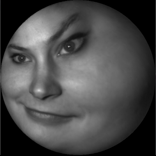
A conformal mapping preserves the angles, and maps infinitesimal circles to the infinitesimal circles, as shown in the top figure.
Riemann Mapping
Riemann Mapping Theorem If $S$ is a topological disk, and $D$ is the planar disk, then there exist conformal mappings from the surface to the disk. All such mappings differ
by a Mobius transformation.
A Mobius transformation conformally maps the unit disk to itself, and has the closed form
\[
\phi(z) = e^{i\theta} \frac{z-z_0}{1-\bar{z}_0 z}, |z| < 1.
\]
Simplicial Forms
Suppose $M$ is a simplicial complex. The simplicial 0-form is a function defined on the vertices, the simplicial 1-form is a linear function defined on the halfedges, the simplicial
2-form is a linear function defined on the oriented faces.
Exterior Differentiation
Suppose $f: V\to R$ is a 0-form, then $df$ is a 1-form,
\[
df( [v_0,v_1]) = f(\partial [v_0,v_1]) = f(v_1) - f(v_0).
\]
Suppose $\omega$ is a 1-form, then $d\omega$ is a 2-form
\[
d\omega([v_0,v_1,v_2]) = \omega (\partial [v_0,v_1,v_2]) = \omega([v_0,v_1]) + \omega([v_1,v_2]) + \omega ([v_2,v_0]).
\]
Wedge Product
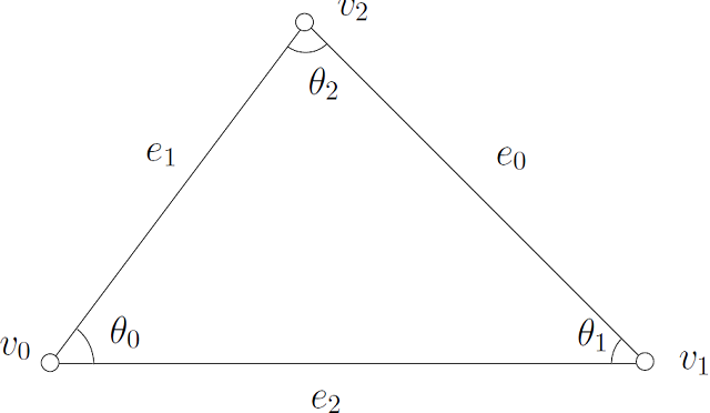
Let $\omega_1$ and $\omega_2$ are two closed 1-forms, the wedge product $\omega_1\wedge \omega_2$ integrated on the triangle $[v_0,v_1,v_2]$ equals to
\[
\int_{[v_0,v_1,v_2]} \omega_1 \wedge \omega_2 = \frac{1}{6}
\left|
\begin{array}{ccc}
\omega_1(e_0) &\omega_1(e_1) &\omega_1(e_2) \\
\omega_2(e_0) &\omega_2(e_1) &\omega_2(e_2) \\
1 & 1 & 1
\end{array}
\right|
\]
Wedge Star Product
The integration of the star wedge product $\omega_1 \wedge {}^*\omega_2$ on $[v_0,v_1,v_2]$ equals to
\[
\int_{[v_0,v_1,v_2]} \omega_1 \wedge {}^*\omega_2 = \frac{1}{2} \sum_{k=0}^2 \cot(\theta_k) \omega_1(e_k) \omega_2(e_k).
\]
Harmonic 1-form
Suppose $\omega$ is a 1-form, $\omega$ is harmonic, if it satisfies
\[
d\omega = 0, \delta \omega = 0,
\]
where
\[
\delta \omega(v_i) = \sum_{[v_i,v_j]\in M} w_{ij} \omega([v_i,v_j]), \forall v_i\in M,
\]
where $w_{ij}$ is the cotangent edge weight.
Diffusion
According to Hodge theory, every cohomological class has a unique harmonic 1-form. Suppose $\omega$ is a closed 1-form, then there exists a unique function (0-form) $f: V\to R$, such that
$\omega + df$ is harmonic. Namely,
\[
d(\omega+df) = d\omega + d^2f = 0, \delta (\omega+ df ) = 0,
\]
The second equation is equivalent to
\[
\sum_{j} w_{ij}(f(v_j) - f(v_i)) = -\sum_j w_{ij}\omega([v_i,v_j]), \forall v_i.
\]
Computational Algorithm
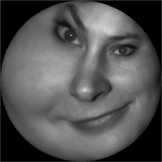
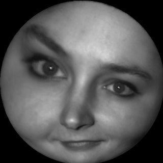
The input mesh $M$ is a topological disk, like a human face mesh.
- Punch a hole in the center of the surface. The surface becomes an annulus, with two boundaries
\[
\partial M = \gamma_0 - \gamma_1.
\]
- Compute the shortest path $\eta$ connecting $\gamma_0$ and $\gamma_1$. Slice the surface along $\eta$ to get a topological disk $\bar{M}$,
\[
\partial \bar{M} = \gamma_0 \cup \eta^{+} \cup \gamma_1 \cup \eta^{-1}.
\]
- Compute the exact harmonoic 1-form $\omega_0$. Compute a harmonic function by solving the following Dirichlet problem,
\[
\left\{
\begin{array}{clc}
\Delta f &=& 0\\
f|_{\gamma_0} & =& 0\\
f|_{\gamma_1} & =& 1
\end{array}
\right.
\]
on the mesh, the discrete harmonic function can be computed
\[
\left\{
\begin{array}{rlcr}
\sum_{j} w_{ij}(f(v_i) - f(v_j)) &=& 0 & \forall v_i \in M\\
f(v_k) & =& 0 & \forall v_k \in \gamma_0\\
f(v_l) & =& 1 & \forall v_l \in \gamma_1\\
\end{array}
\right.
\]
Then the exact harmonic 1-form is given by
\[
\omega_0 = df.
\]
- Assign a function on the sliced mesh $g: \bar{M}\to R$, such that
\[
g(v_i) = \left\{
\begin{array}{cl}
1 & \forall v_i \in \eta^{+}\\
0 & otherwise
\end{array}
\right.
\]
then suppose $e^{+}\in \eta^{+}$, its dual $e^{-}\in \eta^{-}$. Because $dg(e^{+}) = dg(e^{-})=0$, so $dg$ is well defined on the annulus $M$. Define
\[
\tau = dg, \int_{\gamma_0} \tau = 1.
\]
- Diffusion Compute a function $h:V\to R$, such that $\tau + dh$ is harmonic.
\[
\sum_{j} w_{ij} [ \tau( [v_i,v_j] ) + h(v_j) - h(v_i) ] = 0
\]
set $\omega_1 = \tau + dh$.
- Holomorphic 1-form Now we have two harmonic 1-forms $\omega_0$ and $\omega_1$.
\[
\left(
\begin{array}{c}
{}^*\omega_0 \\
{}^*\omega_1
\end{array}
\right) =
\left(
\begin{array}{cc}
\lambda_{00} & \lambda_{01}\\
\lambda_{10} & \lambda_{11}
\end{array}
\right)
\left(
\begin{array}{c}
\omega_0 \\
\omega_1
\end{array}
\right)
\]
We obtain linear system
\[
\left(
\begin{array}{c}
\int_M \omega_0 \wedge {}^*\omega_0 &
\int_M \omega_0 \wedge {}^*\omega_1 \\
\int_M \omega_1 \wedge {}^*\omega_0 &
\int_M \omega_1 \wedge {}^*\omega_1
\end{array}
\right)
=
\left(
\begin{array}{cc}
\int_M \omega_0 \wedge \omega_0 &
\int_M \omega_0 \wedge \omega_1 \\
\int_M \omega_1 \wedge \omega_0 &
\int_M \omega_1 \wedge \omega_1 \\
\end{array}
\right)
\left(
\begin{array}{c}
\lambda_{00} & \lambda_{10}\\
\lambda_{01} & \lambda_{11}
\end{array}
\right)
\]
- Integration Define a function $\phi: \bar{M}\to C$, choose a base vertex $v_0$,
\[
\phi(v_i) = \int_{v_0}^{v_i} \omega_1 + \sqrt{-1} {}^*\omega_1,
\]
- Exponential MapThe final Riemann mapping is the exponential map of $\phi$,
\[
e^{2\pi \sqrt{-1} \phi(v_i)}
\]
- Fill the central hole The central puncture is filled.
- Mobius Transformation The mapping can be further transformed by a Mobius transformation,
\[
z \to e^{\sqrt{-1}\theta} \frac{z-z_0}{1-\bar{z}_0 z}, |z_0 | < 1.
\]
Source Code
The code is written in C++ using VisualStudio on Windows platform. The command pipeline is as follows,
..\..\bin\RiemannMapper.exe -puncture %mesh%.origin.m %mesh%.m
..\..\bin\RiemannMapper.exe -cut %mesh%.m %mesh%
..\..\bin\RiemannMapper.exe -slice %mesh%.cut.m %mesh%.open.m
..\..\bin\RiemannMapper.exe -exact_form %mesh%.m %mesh%
..\..\bin\RiemannMapper.exe -cohomology_one_form_domain %mesh%.m %mesh%.open.m %mesh%_0.dv.m %mesh%_0.dv_uv.m
..\..\bin\RiemannMapper.exe -diffuse %mesh%_0.dv.m %mesh%_0.dv_uv.m %mesh%_0.dv.m %mesh%_0.dv_uv.m
..\..\bin\RiemannMapper.exe -holomorphic_form %mesh%_0.du.m %mesh%_0.dv.m
..\..\bin\RiemannMapper.exe -slit_map holomorphic_form_0.m 0 1 holomorphic.m
..\..\bin\RiemannMapper.exe -integration holomorphic.m %mesh%.open.m %mesh%.uv.m
..\..\bin\RiemannMapper.exe -polar_map %mesh%.m %mesh%.uv.m %mesh%.circ_uv.m
..\..\bin\RiemannMapper.exe -fill_hole %mesh%.circ_uv.m %mesh%.final_uv.m
The source code, testing mesh, texture images and testing scripts can be downloaded here.
A simple triangle mesh viewer can be found here. The command line is
RiemannMapper.exe -riemann_map input.m output.m
In order to view the output
MeshViewer.exe output.m checker.bmp
Contact
If you encounter any problem during the compilation or running the code, please contact the author David Gu at $gu@cs.stonybrook.edu$.